Suppose that 


For 


Let 


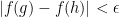
Because a continuous function on a compact set is uniformly continuous (in the sense that there exists a neighbourhood 


This linear functional 


for all
Sean Eberhard's mathematics blog
Suppose that
For
Let
Because a continuous function on a compact set is uniformly continuous (in the sense that there exists a neighbourhood
This linear functional
for all
When I was in high school, I asked several a person, “Why the normal distribution?”. After all, the function 

The real answer that I was looking for but did not appreciate until university was the central limit theorem. For me, the central limit theorem is the explanation of the normal distribution. In any case, the calculation that I attempted was basically a verification of the central limit theorem in a simple case, and it is a testement to the force of the central limit theorem that that simple case is difficult to work out by hand.
In this post, I rectify that calculation that I should have accomplished in high school (with the benefit of hind-sight being the correct factor of 

Consider a “random walk” on 


where each 


where we make the convention that the binomial coefficient is zero when it doesn’t make sense. Hence, if 
By Stirling’s formula, 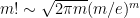
as 
Let 


so 
and by symmetry,
as 
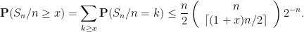
In fact, because the convergence above is geometric,
whence
(This is the Borel–Cantelli lemma.) Thus 
It remains to check the central limit theorem, i.e., to investigate the limiting distribution of 

where 


as
Hence
where 
![{t\in[x,y]}](https://s0.wp.com/latex.php?latex=%7Bt%5Cin%5Bx%2Cy%5D%7D&bg=ffffff&fg=000000&s=0&c=20201002)
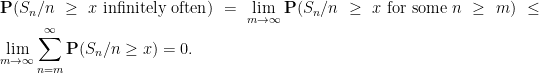
Hence
where the last equality follows from the theorem that continuous functions are Riemann integrable. Thus we have verified the central limit theorem.


![\displaystyle \left|\int_x^y R_n(t)\,d\mu_n(t)\right| \leq \mu_n([x,y]) \max_{x\leq t\leq y} |R_n(t)| \leq (y-x + 2/\sqrt{n})\max_{x\leq t\leq y} |R_n(t)| \rightarrow 0.](https://s0.wp.com/latex.php?latex=%5Cdisplaystyle++%5Cleft%7C%5Cint_x%5Ey+R_n%28t%29%5C%2Cd%5Cmu_n%28t%29%5Cright%7C+%5Cleq+%5Cmu_n%28%5Bx%2Cy%5D%29+%5Cmax_%7Bx%5Cleq+t%5Cleq+y%7D+%7CR_n%28t%29%7C+%5Cleq+%28y-x+%2B+2%2F%5Csqrt%7Bn%7D%29%5Cmax_%7Bx%5Cleq+t%5Cleq+y%7D+%7CR_n%28t%29%7C+%5Crightarrow+0.+&bg=ffffff&fg=000000&s=0&c=20201002)

